
딥러닝 MNIST 실습_캐글 Sign Language 데이터셋
1. 딥러닝 MNIST 실습
· 영어 알파벳 수화 데이터셋
(※ 링크 : https://www.kaggle.com/datamunge/sign-language-mnist)
1) 데이터셋 다운로드
import os
os.environ['KAGGLE_USERNAME'] = '<username>' # username
os.environ['KAGGLE_KEY'] = '<key>' # key
!kaggle datasets download -d datamunge/sign-language-mnist
!unzip sign-language-mnist.zip
2) 패키지 로드
from tensorflow.keras.models import Model
from tensorflow.keras.layers import Input, Dense
from tensorflow.keras.optimizers import Adam, SGD
import numpy as np
import pandas as pd
import matplotlib.pyplot as plt
import seaborn as sns
from sklearn.model_selection import train_test_split
from sklearn.preprocessing import StandardScaler
from sklearn.preprocessing import OneHotEncoder
3) 데이터셋 로드
# 1) 트레이닝셋
train_df = pd.read_csv('sign_mnist_train.csv')

train_df.head()
# 2) 테스트셋
test_df = pd.read_csv('sign_mnist_test.csv')

test_df.head()
4) 라벨 분포
9=J or 25=Z 는 동작이 들어가므로 제외, 총 24개의 라벨
plt.figure(figsize=(16, 10))
sns.countplot(train_df['label'])
plt.show()
5) 전처리
입력과 출력 나누기
train_df = train_df.astype(np.float32)
x_train = train_df.drop(columns=['label'], axis=1).values       # label만 제외
y_train = train_df[['label']].values                            # label만 포함

test_df = test_df.astype(np.float32)
x_test = test_df.drop(columns=['label'], axis=1).values
y_test = test_df[['label']].values

# 트레이닝, 테스트셋 모양 확인하기
print(x_train.shape, y_train.shape)
print(x_test.shape, y_test.shape)

"""
(27455, 784) (27455, 1)
(7172, 784) (7172, 1)
"""
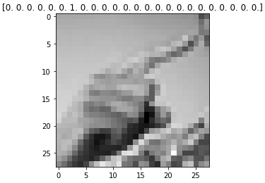
6) 데이터 미리보기
index = 1
plt.title(str(y_train[index]))
plt.imshow(x_train[index].reshape((28, 28)), cmap='gray')       # 픽셀이 일자로 늘어서 있기 때문에 reshape를 해준다.
plt.show()          # onehot encoding 전 -> [6.], 후 -> [0. 0. 0. 0. 0. 0. 1. 0. ....]
7) One-hot encoding
encoder = OneHotEncoder()
y_train = encoder.fit_transform(y_train).toarray()
y_test = encoder.fit_transform(y_test).toarray()

print(y_train.shape)

"""
(27455, 24)
"""
8) 일반화
: 이미지 데이터는 픽셀이 0-255 사이의 정수(unsigned integer 8bit = uint8)로 되어 있으므로 255로 나누어 0-1 사이의 소수점 데이터(floating point 32bit = float32)로 바꾸어 일반화 시킬 수 있다.
x_train = x_train / 255.        # 이미지데이터의 픽셀은 0~255까지의 정수로 되어있기 때문에 255로 나눈다.
x_test = x_test / 255.          # 이를 통해 0~1사이의 값으로 바꾸어줄 수 있다.
9) 네트워크 구성
input = Input(shape=(784,))                           # input node : 784개
hidden = Dense(1024, activation='relu')(input)        # 순차적으로 input -> hidden .. 레이어를 넣는다.
hidden = Dense(512, activation='relu')(hidden)
hidden = Dense(256, activation='relu')(hidden)
output = Dense(24, activation='softmax')(hidden)      # 26개의 알파벳중 j, z를 뺀 24개 아웃풋
                                                      # activation은 다항 논리회귀와 같이 softmax사용
model = Model(inputs=input, outputs=output)           # Functional API 사용

model.compile(loss='categorical_crossentropy', optimizer=Adam(lr=0.001), metrics=['acc'])

model.summary()     # 모델 요약 출력
10) 학습
history = model.fit(
    x_train,
    y_train,
    validation_data=(x_test, y_test), # 검증 데이터를 넣어주면 한 epoch이 끝날때마다 자동으로 검증
    epochs=20 # epochs 복수형으로 쓰기!
)
11) 학습결과 그래프
# loss 히스토리 확인
plt.figure(figsize=(16, 10))
plt.plot(history.history['loss'])
plt.plot(history.history['val_loss'])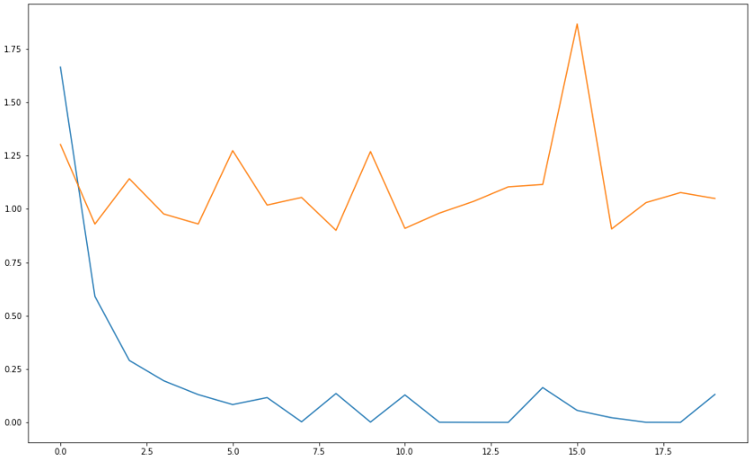
# 정확도 히스토리 확인
plt.figure(figsize=(16, 10))
plt.plot(history.history['acc'])
plt.plot(history.history['val_acc'])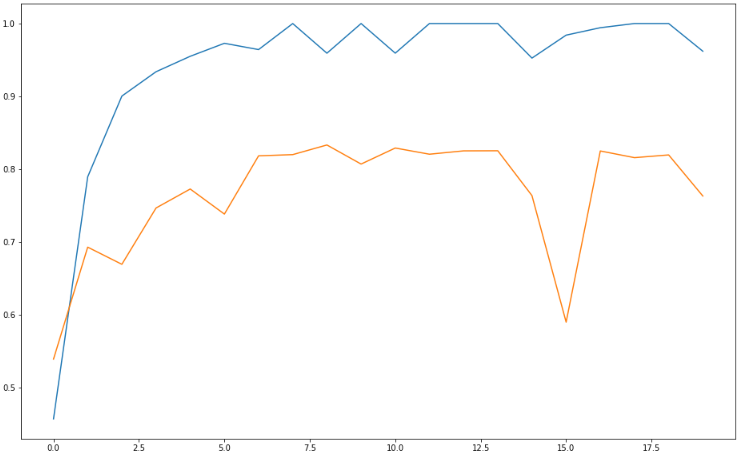
반응형
'DataScience > 머신러닝' 카테고리의 다른 글
| 머신러닝 :: 딥러닝_전이학습, 순환신경망(RNN), 생성적 적대 신경망(GAN) (0) | 2022.10.13 |
|---|---|
| 머신러닝 :: 합성곱 신경망(CNN, Convolutional Neural Networks) (0) | 2022.10.13 |
| 머신러닝 :: 딥러닝 XOR 예측 실습(이진 논리회귀, MLP, keras functional API) (0) | 2022.10.13 |
| 머신러닝 :: 딥러닝 주요 개념(배치, 활성화 함수, 과적합, 앙상블) (0) | 2022.10.13 |
| 머신러닝 :: 다항 논리회귀(Logistic Regression)_와인 종류 예측 (0) | 2022.10.12 |


댓글